The realm of spatial machine learning is gaining traction, especially with the advancements in the R programming language. This article marks the beginning of a detailed blog series dedicated to spatial machine learning using R. The objective is to delve into the capabilities of R in handling machine learning tasks that incorporate spatial variables, which is a crucial factor in many real-world scenarios.

R offers a rich array of packages designed for machine learning, making it a suitable choice for tackling tasks in a spatial context. A fundamental principle of spatial machine learning is that observations closer in proximity tend to exhibit greater similarity than those located farther apart. This necessitates a unique approach when developing machine learning models, as spatial relationships can significantly influence results.

In this initial post, we aim to compare three of the most prominent machine learning frameworks available in R: caret, tidymodels, and mlr3. Through a straightforward example, we will illustrate how to utilize these frameworks for a specific spatial machine learning task while highlighting the differences in their workflows. The intent is to provide readers with a clear understanding of the spatial machine learning process and how these various frameworks can be employed to achieve similar objectives.

The scenario we will explore involves predicting the temperature across different regions in Spain, utilizing a set of covariates. For this purpose, we have two datasets: the first, named temperature_train, encompasses temperature measurements from 195 distinct locations throughout Spain. The second dataset, predictor_stack, consists of various covariates that will facilitate our temperature predictions. These covariates include crucial variables such as population density (popdens), distance to the coast (coast), and elevation (elev), among others.

To start with, we load the necessary libraries and datasets. The temperature measurement dataset can be accessed using the following command:

library(terra)library(sf)train_points <- sf::read_sf("https:predictor_stack <- terra::rast("https:
With the datasets loaded, we proceed to extract the relevant covariate values corresponding to our training points. We will utilize a subset of fourteen covariates to forecast the temperature:
predictor_names <- names(predictor_stack)[1:14]temperature_train <- terra::extract(predictor_stack[[predictor_names]], train_points, bind = TRUE) >| sf::st_as_sf()
At this stage, our temperature_train dataset is fully prepared, containing both the temperature measurements and the covariate values for each location, thereby making it suitable for modeling.
Next, we delve into loading the frameworks necessary for our modeling tasks. Each framework requires loading specific packages:
library(caret) # for modelinglibrary(blockCV) # for spatial cross-validationlibrary(CAST) # for area of applicabilitylibrary(tidymodels) # metapackage for modelinglibrary(spatialsample) # for spatial cross-validationlibrary(waywiser) # for area of applicabilitylibrary(vip) # for variable importance (used in AOA)library(mlr3verse) # metapackage for mlr3 modelinglibrary(mlr3spatiotempcv) # for spatial cross-validationlibrary(CAST) # for area of applicabilitylgr::get_logger("mlr3")$set_threshold("warn")
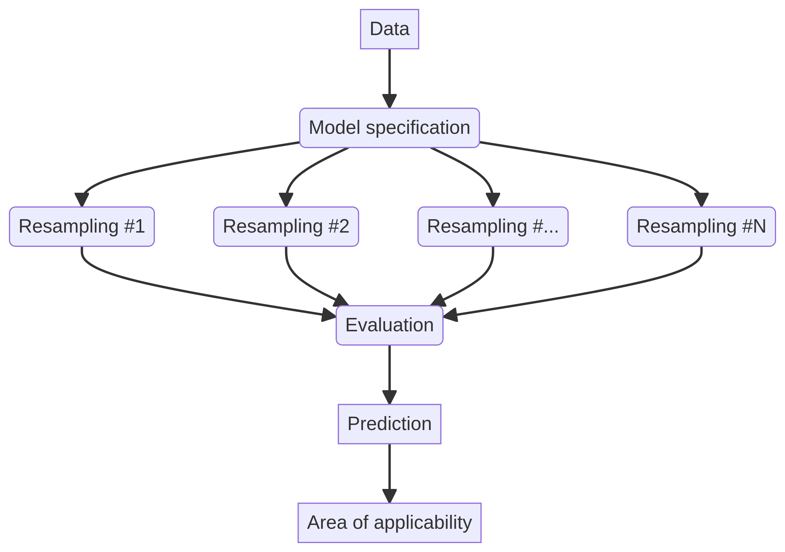
Upon loading the necessary packages, it is essential to define the modeling workflow. Each framework has its distinct approach to model specification, encompassing aspects such as model definition, resampling methods, and hyperparameter values. In our example, we will employ random forest models, specifically using the ranger package. The hyperparameters are defined as follows:
    
mtry: The number of variables randomly sampled as candidates at each split is set to 8.
    
splitrule: The splitting rule utilized is extratrees.
    
min.node.size: The minimum size of terminal nodes is defined as 5.
We will implement a spatial cross-validation strategy with 5 folds. This involves partitioning the data into several spatial blocks, with each block assigned to a specific fold. The model is then trained on a collection of blocks from the training set while being evaluated on the remaining blocks. It is noteworthy that each framework has its unique way of defining the resampling method, resulting in slight variations in implementation and folds.
For the caret framework, we establish the hyperparameter grid through the expand.grid() function and configure the resampling method using the trainControl() function. To ensure spatial cross-validation, the blockCV package is utilized to create the folds, which are subsequently passed to the trainControl() function:
set.seed(22) # hyperparameterstn_grid <- expand.grid(mtry = 8, splitrule = "extratrees", min.node.size = 5)spatial_blocks <- blockCV::cv_spatial(temperature_train, k = 5, hexagon = FALSE, progress = FALSE)
We then extract training and testing identifiers from the spatial blocks:
train_ids <- lapply(spatial_blocks$folds_list, function(x) x[[1]])test_ids <- lapply(spatial_blocks$folds_list, function(x) x[[2]])tr_control <- caret::trainControl(method = "cv", index = train_ids, indexOut = test_ids, savePredictions = TRUE)
In the tidymodels framework, we initiate the process by specifying the modeling formula using the recipe() function. We then define the model using a function from the parsnip package, which includes the hyperparameters. The model and recipe are combined into a workflow using the workflow() function, followed by the definition of the resampling method through the spatial_block_cv() function from the spatialsample package:
set.seed(22)form <- as.formula(paste0("temp ~ ", paste(predictor_names, collapse = " + "))) recipe <- recipes::recipe(form, data = temperature_train)rf_model <- parsnip::rand_forest(trees = 100, mtry = 8, min_n = 5, mode = "regression") >| set_engine("ranger", splitrule = "extratrees", importance = "impurity")workflow <- workflows::workflow() >| workflows::add_recipe(recipe) >| workflows::add_model(rf_model)block_folds <- spatialsample::spatial_block_cv(temperature_train, v = 5)spatialsample::autoplot(block_folds)
In mlr3, we define the task using the as_task_regr_st() function, which specifies the target variable and data. The model is defined using the lrn() function, which outlines the model type and hyperparameters. Additionally, the resampling method is specified using the rsmp() function:
set.seed(22)task <- mlr3spatiotempcv::as_task_regr_st(temperature_train, target = "temp")learner <- mlr3::lrn("regr.ranger", num.trees = 100, importance = "impurity", mtry = 8, min.node.size = 5, splitrule = "extratrees")resampling <- mlr3::rsmp("spcv_block", folds = 5, cols = 10, rows = 10)
As we move into the modeling phase, each framework showcases its own methods for model training. The primary function in the caret package is train(), which accommodates the formula, data, model type, tuning grid, training control, and additional parameters like the number of trees. This function automatically conducts resampling and hyperparameter tuning when applicable:
model_caret <- caret::train(temp ~ ., data = st_drop_geometry(temperature_train), method = "ranger", tuneGrid = tn_grid, trControl = tr_control, num.trees = 100, importance = "impurity")model_caret_final <- model_caret$finalModel
For tidymodels, the fit_resamples() function is employed, taking the previously established workflow and resampling folds. The fit_best() function is then utilized to fit the optimal model based on the resampling outcomes:
rf_spatial <- tune::fit_resamples(workflow, resamples = block_folds, control = tune::control_resamples(save_pred = TRUE, save_workflow = TRUE))model_tidymodels <- fit_best(rf_spatial)
In mlr3, the resample() function is applied to the task, learner, and resampling method. To obtain the final model, the train() function is called on the previously defined task and learner:
model_mlr3 <- mlr3::resample(task = task, learner = learner, resampling = resampling)learner$train(task)
After successfully training the models, its vital to evaluate their performance. We will employ two widely used metrics for regression tasks: the root mean square error (RMSE) and the coefficient of determination (R). Both metrics are calculated by default in caret, with the performance metrics stored in the results object of the model:
model_caret$results
Similarly, in tidymodels, the metrics are derived from the resampling results using the collect_metrics() function:
tune::collect_metrics(rf_spatial)
For mlr3, we define the measures we wish to calculate using the msr() function and then utilize the aggregate() method to compute the selected performance metrics:
my_measures <- c(mlr3::msr("regr.rmse"), mlr3::msr("regr.rsq"))model_mlr3$aggregate(measures = my_measures)
Ultimately, our goal is to forecast the temperature across Spain based on the covariates from the predictor_stack dataset. Thus, we aim to generate a map depicting the predicted temperature values nationwide. The predict() function from the terra package enables us to make model predictions on the new raster data:
pred_caret <- terra::predict(predictor_stack, model_caret, na.rm = TRUE)plot(pred_caret)pred_tidymodels <- terra::predict(predictor_stack, model_tidymodels, na.rm = TRUE)plot(pred_tidymodels)pred_mlr3 <- terra::predict(predictor_stack, learner, na.rm = TRUE)plot(pred_mlr3)
An important consideration is the area of applicability (AoA), a method that assesses the extent of the input space that is analogous to the training data. This tool is invaluable for evaluating model performance and identifying regions where the model predictions may be applicable. Areas lying outside the AoA are deemed out of the model's applicability domain, necessitating cautious interpretation of predictions made in those regions.
The original implementation of the AoA method is found within the CAST package, which extends the capabilities of the caret package. The AoA is computed using the aoa() function, which takes new data (the covariates) and the model as inputs:
AOA_caret <- CAST::aoa(newdata = predictor_stack, model = model_caret, verbose = FALSE)plot(AOA_caret$AOA)
For tidymodels, the AoA method is executed via the waywiser package, where the ww_area_of_applicability() function requires training data and variable importance as inputs:
model_aoa <- waywiser::ww_area_of_applicability(st_drop_geometry(temperature_train[, predictor_names]), importance = vip::vi_model(model_tidymodels))AOA_tidymodels <- terra::predict(predictor_stack, model_aoa)plot(AOA_tidymodels$aoa)
Meanwhile, for mlr3 models, the CAST package can also be utilized to calculate the AoA, requiring various parameters such as a covariance raster, training data, relevant variables, weights, and cross-validation folds:
rsmp_cv <- resampling$instantiate(task)AOA_mlr3 <- CAST::aoa(newdata = predictor_stack, train = as.data.frame(task$data()), variables = task$feature_names, weight = data.frame(t(learner$importance())), CVtest = rsmp_cv$instance[order(row_id)]$fold, verbose = FALSE)plot(AOA_mlr3$AOA)
In conclusion, this blog post has provided a comparative analysis of three of the leading machine learning frameworks in R: caret, tidymodels, and mlr3. We have explored how to use these frameworks for spatial machine learning tasks, covering aspects such as model specification, training, evaluation, prediction, and the area of applicability. While there is considerable overlap in the functionalities offered by these frameworks, they also exhibit distinct design philosophies and implementations. For instance, caret offers a more consistent and concise interface, but this comes with limited flexibility. In contrast, tidymodels and mlr3 are more modular and flexible, allowing for intricate workflows and customizations, although they also entail a steeper learning curve.
There are numerous additional steps that can be incorporated into the workflow presented, such as feature engineering, variable selection, hyperparameter tuning, and model interpretation. In forthcoming blog posts, we will delve deeper into these three frameworks and introduce other packages that can be harnessed for spatial machine learning in R.
Reuse CC BY 4.0 Citation BibTeX citation: @online{nowosad2025, author = {Nowosad, Jakub}, title = {Spatial Machine Learning with {R:} Caret, Tidymodels, and Mlr3}, date = {2025-04-30}, url = {https:
To attribute this work, please cite as follows: Spatial Machine Learning with R: Caret, Tidymodels, and Mlr3. April 30, 2025. Nowosad, Jakub. 2025. April 30, 2025. 
                    

                          R-bloggers.com 
                    
                    

                         2025-04-30
                    
                    

                         
Hana Takahashi